Hi - Dave here.
Happy Friday!
In my last email, I talked about how the FILTER function is great for finding all matches, and I shared a simple example where we used FILTER to find all records in the "Red" group.
What you might not realize is that you can use FILTER to find records based on information that is
not part of the data. In other words, you can manipulate the logical test to generate the information you need to find things.
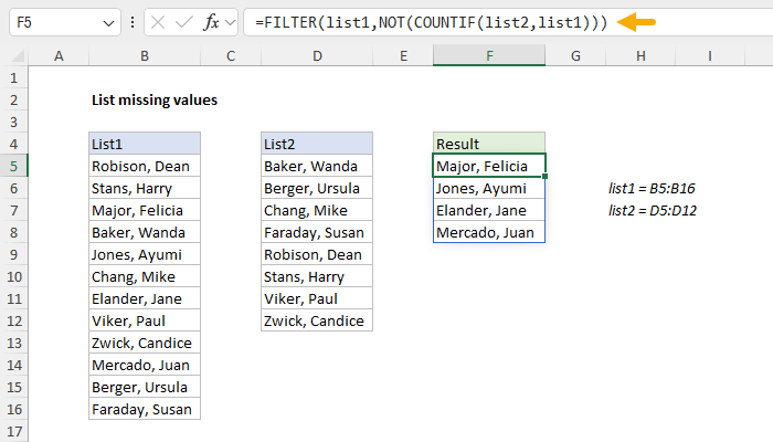
For example, the worksheet below contains two lists of names. The first list is people who were
invited to an event. The second list is people who actually
attended the event. The goal is to find people who were invited but did
not attend the event. That is, we want to find "missing" people. But notice we have no field called "Missing" to filter on. However, we can create the missing info with a formula like this in cell F5:
=FILTER(list1,NOT(COUNTIF(list2,list1)))
[
Download the workbook and read the full explanation]
In a nutshell, COUNTIF counts people in list2 who also appear in list1. Then, the NOT function reverses the count to flag those people who are missing.
I like the COUNTIF + NOT pattern because it is intuitive. But note that it will fail if list2 is an
array and not a proper
range. This is a known limitation of all the *IFS functions. A good workaround is to use a formula based on ISNA + XMATCH instead. The article above explains both formulas in detail.
Note: FILTER requires Excel 2021+ or Excel 365.
Excel formulas
We maintain a list of over 1000 working formulas
here.
If you need more structure, we also offer
paid training.
Have a great weekend!
Dave
The Exceljet newsletter is free and sent weekly on Fridays. Each week, I take a detailed look at a specific Excel formula or function. Sign up on our home page.