Hi - Dave here.
Happy Friday!
This week, I want to introduce TRIMRANGE, a geeky but cool new function that solves an important problem in Excel – how to create a simple dynamic range with a formula.
A dynamic range is a range that expands and contracts with your data. This is a tricky problem and, in the past, it required a complicated formula like this:
=OFFSET(B5,0,0,COUNTA($B$5:$B$100),COUNTA($B$4:$Z$4))
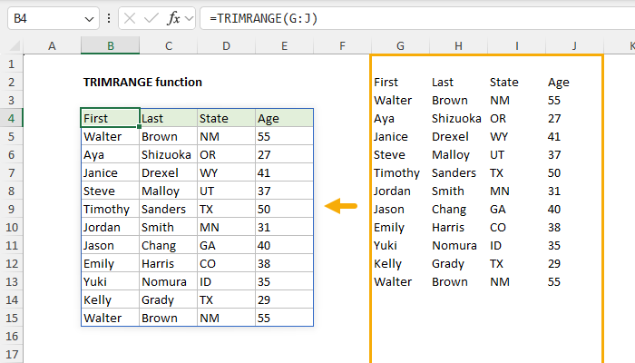
With TRIMRANGE, you can use a simple formula like this:
=TRIMRANGE(range)
In fact, you can even use dangerously large ranges like G:J, and TRIMRANGE will happily chop them down to size, as you can see in the workbook below:
[
Download the workbook and read the full explanation]
The beauty of TRIMRANGE is that it will track the data in a worksheet as it changes. When data is added or removed, the range will automatically adapt, with no need to adjust cell references manually. This means you can feed the result from TRIMRANGE into other formulas, and they will always use the latest data to calculate results. For this reason, TRIMRANGE is a good option for creating a dynamic range for any data that changes on a regular basis, like order data, signup lists, web traffic, bank transactions, etc. You can even use TRIMRANGE to populate a dropdown list.
Note: TRIMRANGE is a new function in Excel and is only available in Excel 365 for now.
What about Excel Tables?
You might wonder about Excel Tables, can't they also create a dynamic range? Yes, Excel Tables are an excellent way to create a dynamic range in a workbook. However, Excel Tables have some limitations in Excel that mean they don't always work in every situation. TRIMRANGE gives us a simple alternative.
Excel formulas
We maintain a list of over 1000 working formulas
here.
If you need more structure, we also offer
video training.
Have a great weekend!
Dave
The Exceljet newsletter is free and sent weekly on Fridays. Each week, I take a detailed look at how to solve a specific problem with an Excel formula. You can sign up on our home page.