Hi - Dave here.
Happy Friday!
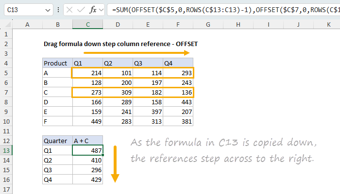
Here's a tricky problem in Excel that many users struggle with. Your data runs across, with quarters in columns C, D, E, and F. Your summary runs down, one quarter per row. Your goal is to total sales for products A and C in each quarter, as shown below.
You write a formula for the first quarter:
| =SUM(C5,C7) |
Then you drag it down, and Excel gives you =SUM(C6,C8). But what you want is =SUM(D5,D7). How can you build a cell reference that will move across columns as you copy a formula down? Should you use a reference like $C$5, $C5, or C$5?
No. No normal reference will work. This is because relative references change only in the direction you copy. When you copy a formula down, the row numbers will change, but the column letters never will.
The solution is to lock each reference to a starting point, and move it with a counter. You can see how this works in the worksheet below, where the formula in C13, copied down, is:
| =SUM(OFFSET($C$5,0,ROWS(C$13:C13)-1),OFFSET($C$7,0,ROWS(C$13:C13)-1)) |
Download the workbook and read the full explanation
Unless you're a formula pro, you probably don't like this formula :) But honestly, it's not too bad once you understand how OFFSET works. Inside the SUM function, we still have two references, both created by the OFFSET function. OFFSET starts from an origin, then "offsets" a certain number of rows and/or columns. The rows offset is zero, since we don't want rows to change. The tricky part is the columns offset: ROWS(C$13:C13)-1.
ROWS(C$13:C13) works like a counter. It returns 1, 2, 3, and 4 as the formula is copied down, because the range expands by one row each time. Subtracting 1 makes the offsets 0, 1, 2, and 3, so the first formula stays in column C, and the next ones step to D, E, and F.
Note that OFFSET is volatile (it recalculates every time the worksheet changes), which can degrade performance in a large workbook. If performance becomes a problem, you can switch to INDEX, as explained on the page.
Also, in newer versions of Excel, you can skip copying altogether. This clever formula gives the same result in one step:
| =TRANSPOSE(C5:F5+C7:F7) |
Which one would you use?
Note: The OFFSET and INDEX formulas work in any version of Excel. The TRANSPOSE option requires Excel 2021 or later because it spills results onto the worksheet.
Keeping Exceljet going
The internet as we know it is getting crushed by AI. Many websites have lost more than half their traffic, making their future uncertain. If you find Exceljet helpful, you can support the site and go ad-free with the Exceljet Lifetime Pass. One payment, no subscription, and ads are gone forever.
Excel formulas
We maintain a list of over 1000 working formulas here.
If you need more structure, we also offer video training.
Have a great weekend!
Dave
The Exceljet newsletter is free and sent weekly on Fridays. Each week, I take a detailed look at a specific Excel formula or function. Sign up on our home page.

Exceljet
P.O. Box 4804
Salt Lake City, UT 84110
Copyright © 2026 Exceljet, All rights reserved.
You received this email because you are subscribed to our newsletter.
To unsubscribe, click the link below.