Hi - Dave here.
Happy Friday!
Last week, I shared a
worksheet to calculate US income taxes in brackets, updated with 2024 tax rates.
One of the techniques I used is a "step-based lookup formula". This is a clever way to navigate data that follows a pattern. Unless you've seen this trick before, you might not understand how it works, so I have a simpilfied example to explain the idea.
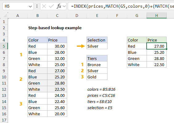
In the worksheet below, we have three tiers of pricing (Bronze, Silver, and Gold) listed in columns B and C. We want to look up the correct pricing based on the selected tier in cell E5, but the tier is not a column in the lookup table.
The solution in cell H5 is an INDEX and MATCH formula modified to "step" through the tiers:
=INDEX(prices,MATCH(G5,colors,0)+(MATCH(selection,tiers,0)-1)*4)
[
Download the workbook and read the full explanation]
At the core, this is a normal INDEX and MATCH formula: MATCH looks up the position of the color in G5, and INDEX returns the price at that position. But notice the second MATCH function, which handles the "step" needed to get pricing for the selected tier. Read the full explanation at the link above. Then download the workbook to try it out yourself.
Note: this formula will work in all versions of Excel.
Excel formulas
We maintain a list of over 1000 working formulas
here.
If you need more structure, we also offer
video training.
Have a great weekend!
Dave
The Exceljet newsletter is free and sent weekly on Fridays. Each week, I take a detailed look at how to solve a specific problem with an Excel formula. You can sign up on our home page.