Hi - Dave here.
Happy Friday!
Last week, I introduced the GROUPBY function. This week, I want to introduce GROUPBY's big brother, the PIVOTBY function.
PIVOTBY works just like GROUPBY, with one big difference: while GROUPBY can group by rows only, PIVOTBY can group by rows
and columns.
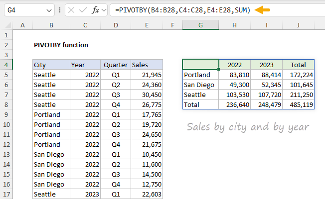
You can see how it works in the example below, where PIVOTBY is summarizing Sales by City and by Year. The formula in G4 looks like this:
=PIVOTBY(B4:B28,C4:C28,E4:E28,SUM)
[
Download the workbook and read the full explanation]
The entire table is created with one formula. Sales by city are calculated in rows, and sales by year are calculated in columns. Unlike a Pivot Table, PIVOTBY does not need to be refreshed; you will always see the latest information if the source data changes. On the other hand, PIVOTBY does not apply any formatting, so that part is entirely manual. Check the link above for a detailed explanation of how to use PIVOTBY and download the workbook that contains all examples and data.
Note: PIVOTBY and GROUPBY are only available in Excel 365.
The end of Pivot Tables?
I don't think so. Even though GROUPBY and PIVOTBY can do many things a Pivot Table can do, Pivot Tables are still a better way to explore data quickly and interactively, and a proven tool to automate regular reports. Plus, Pivot Tables have a big advantage: they automatically apply formatting. For a good overview of Pivot Tables (with sample data),
see this article.
The chatbot is waiting to help you
Got a question about Excel? Try the
Exceljet Chatbot. It gets a little bit smarter each week 🙂
Excel formulas
We maintain a list of over 1000 working formulas
here.
If you need more structure, we also offer
video training.
Have a great weekend!
Dave
The Exceljet newsletter is free and sent weekly on Fridays. Each week, I take a detailed look at a specific Excel formula or function. Sign up on our home page.